

Understanding The Encoder (Part II)
Decoding the Encoder: A Deep Dive into Transformer Architecture

This article is the second part of a three-part deep dive into one of the most revolutionary AI architectures of our time:
Transformers
Here’s what’s coming your way:
✅ Week 1: Understanding the Transformers architecture → Link
✅ Week 2: The Encoder → Link
🔜 Week 3: The Decoder → Coming next 28th June 2026
Understanding the Encoder - Part II
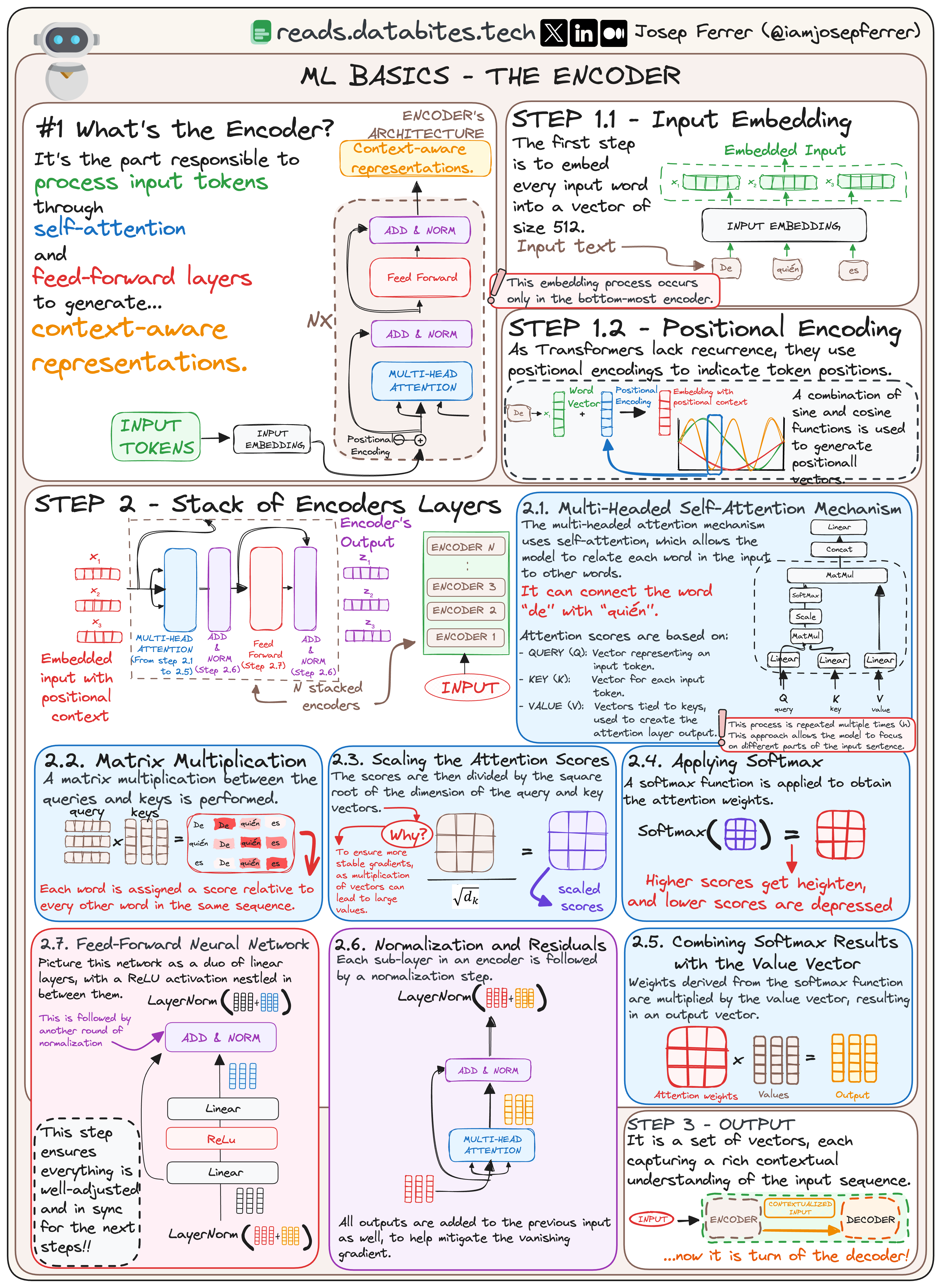
The encoder is a fundamental component of the Transformer architecture.
The primary function of the encoder is:
To transform the input tokens into contextualized representations.
Unlike earlier models that processed tokens independently, the Transformer encoder captures the context of each token in relation to the entire sequence.
Its structure consists of the following elements:

Multi-Head Self-Attention Layer
Layer Normalization (applied twice per layer)
Feed-Forward Neural Network
Before starting, here you have the full-resolution cheatsheet 👇🏻
And now… let’s break it down!
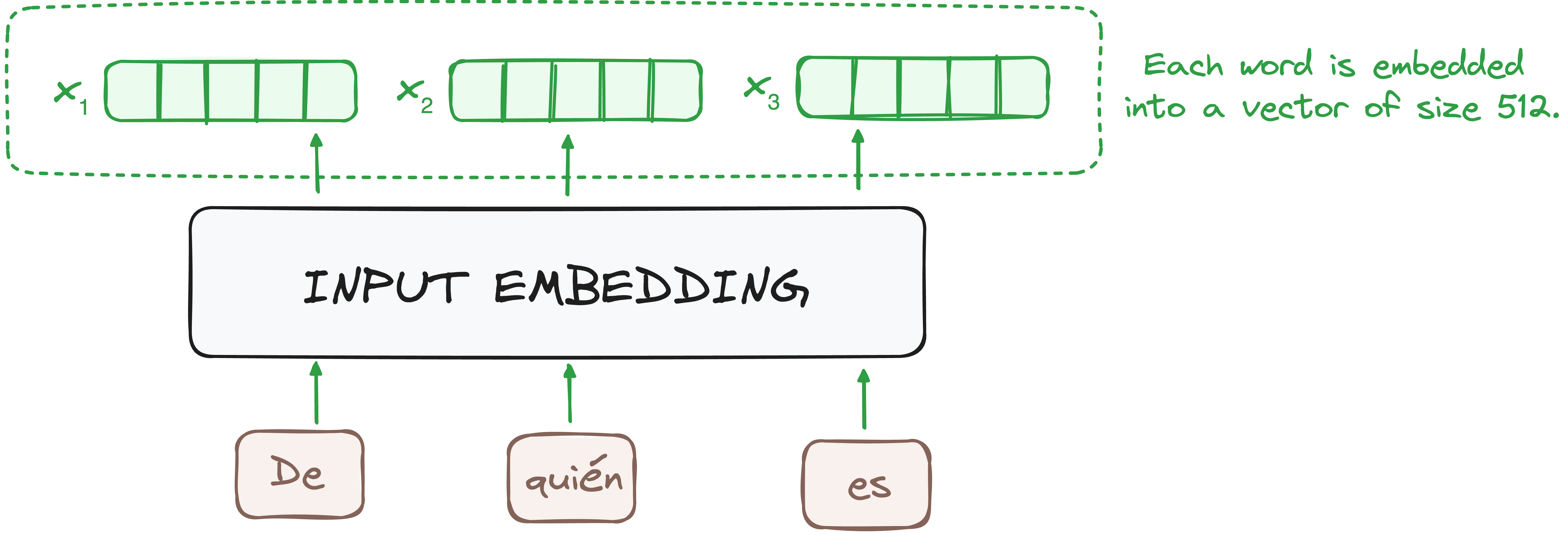
STEP 1 - Input Embeddings
The embedding process occurs only in the bottom-most encoder layer. Remember that the encoder consists of multiple identical layers (six in the original model).
(💡 Missed Part 1? Check it out to get the full picture of how the Transformer works!)

At this stage, the input tokens—whether words or subwords—are converted into dense numerical vectors using embedding layers. These embeddings capture the semantic meaning of the tokens, allowing the model to process them in a continuous space rather than as discrete symbols.
Each encoder receives a list of fixed-size vectors (typically 512-dimensional in the original Transformer). In the first encoder, these are word embeddings, whereas in subsequent encoders, they are the transformed outputs from the previous encoder layer.
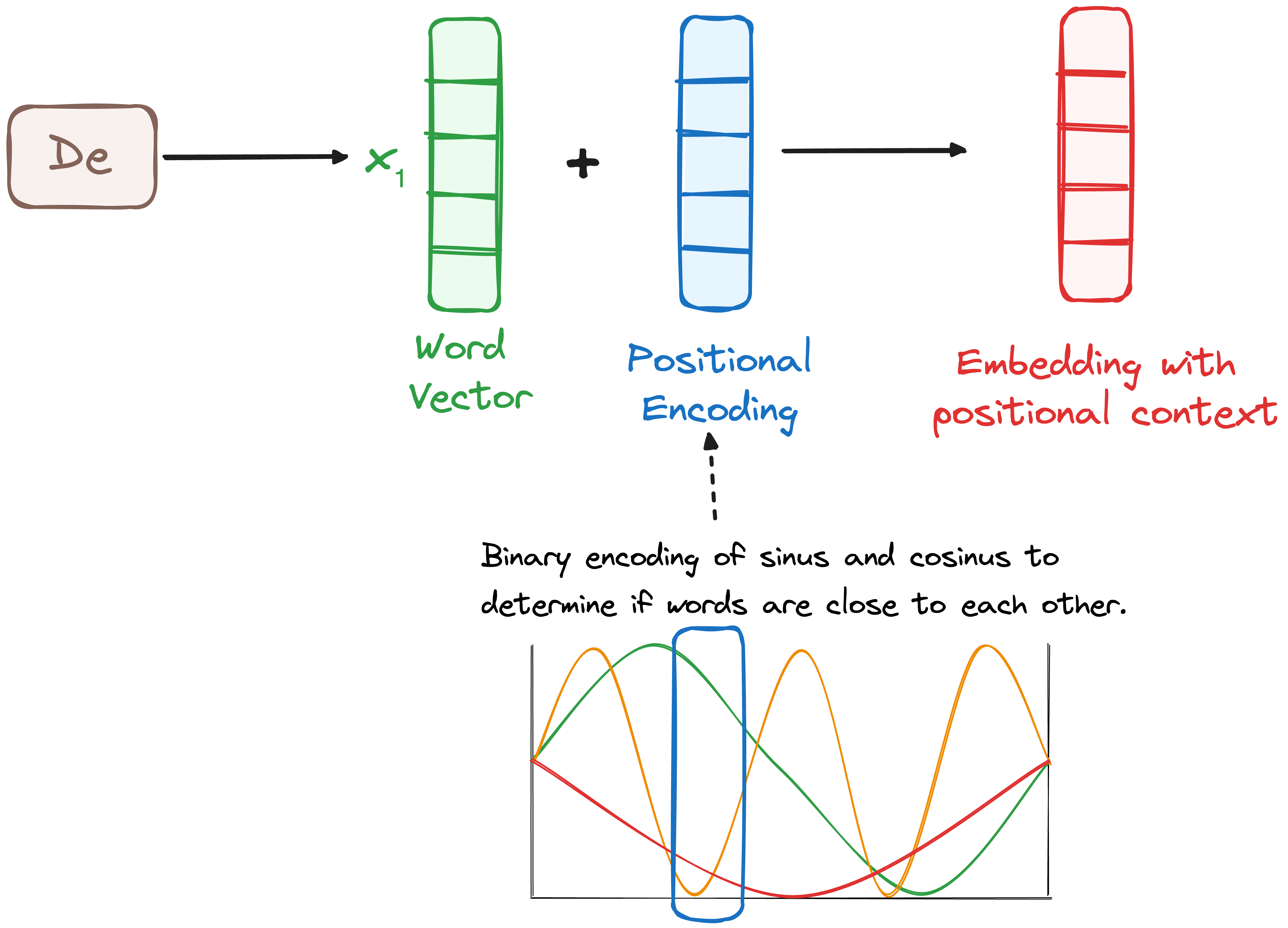
STEP 2 - Positional Encoding
Unlike RNNs, which inherently capture order due to their sequential nature, Transformers lack a built-in notion of token position. To overcome this, they use positional encodings, which are added to the input embeddings to provide information about token order.
These encodings are generated using sine and cosine functions at different frequencies, allowing them to represent positional information independent of sentence length. Each dimension in the positional encoding corresponds to a unique frequency, ensuring that every token position has a distinct representation with values ranging between -1 and 1.
By integrating these encodings, the model understands token positions without relying on recurrence, maintaining efficiency while capturing sequential dependencies.
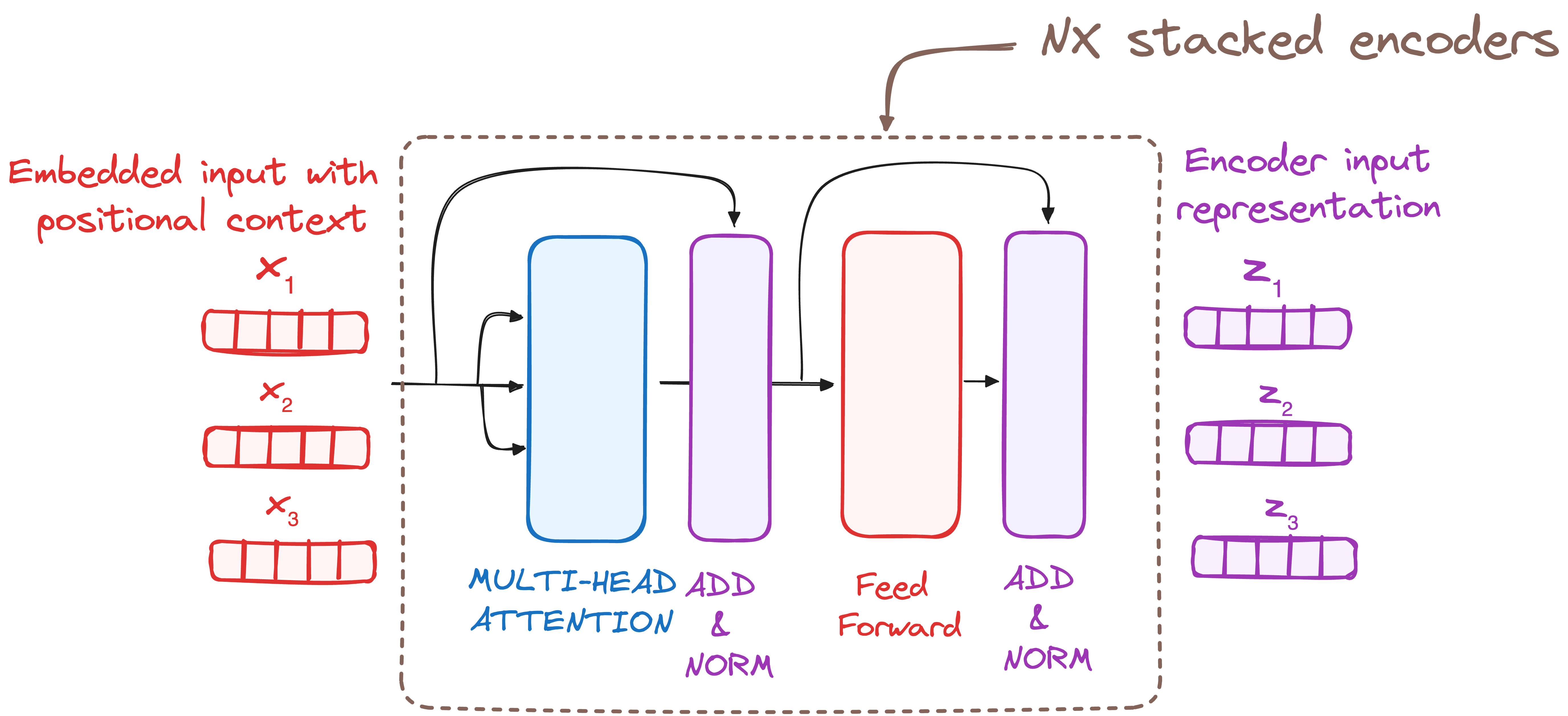
STEP 3 - Stack of Encoder Layers
Each encoder layer transforms the input sequence into a more abstract, context-aware representation.
Each encoder layer consists of two core submodules:
Multi-Head Self-Attention Mechanism (enabling the model to focus on relevant tokens)
Feed-Forward Neural Network (enhancing learned features)
Each submodule is wrapped in residual connections and followed by layer normalization, improving training stability and gradient flow.
STEP 3.1 Multi-Headed Self-Attention Mechanism
In the encoder, the multi-headed attention utilizes a specialized attention mechanism known as self-attention. It allows each token to attend to every other token in the sequence, enabling the model to capture contextual relationships effectively.
This approach enables the models to relate each word in the input with other words. For instance, in a given example, the model might learn to connect the word “are” with “you”.
Each token is projected into three vectors:
Query (Q): Represents a specific word or token from the input sequence in the attention mechanism.
Key (K): Represents another vector in the attention mechanism, corresponding to each word or token in the input sequence.
Value (V): Each value is associated with a key and is used to construct the output of the attention layer. When a query and a key match well (which means that they have a high attention score) the corresponding value is emphasized in the output.
Then the system computes Attention Scores.
The attention score between a query and a key is computed using a dot product.
Higher scores indicate a stronger relationship between tokens.
The detailed architecture goes as follows:
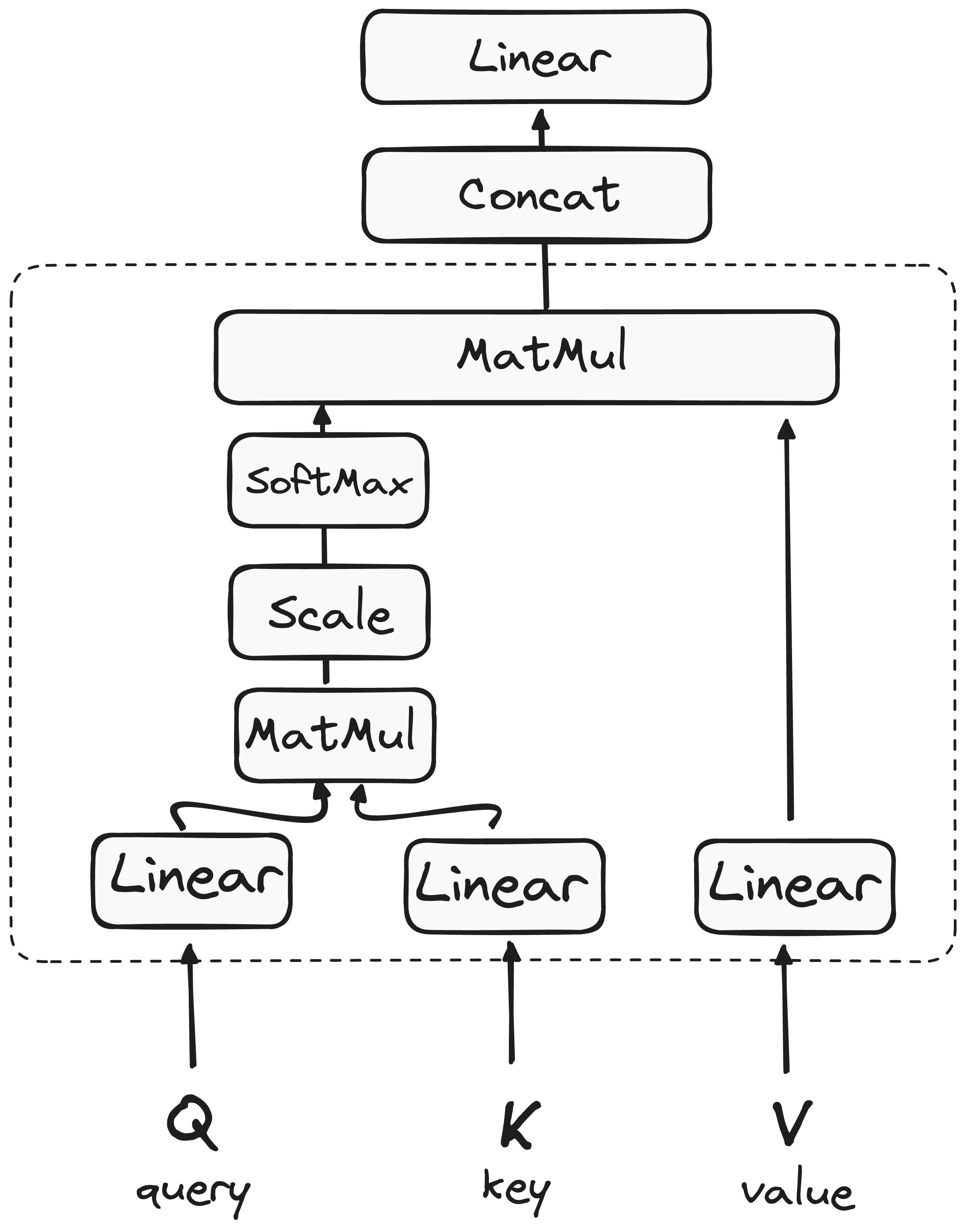
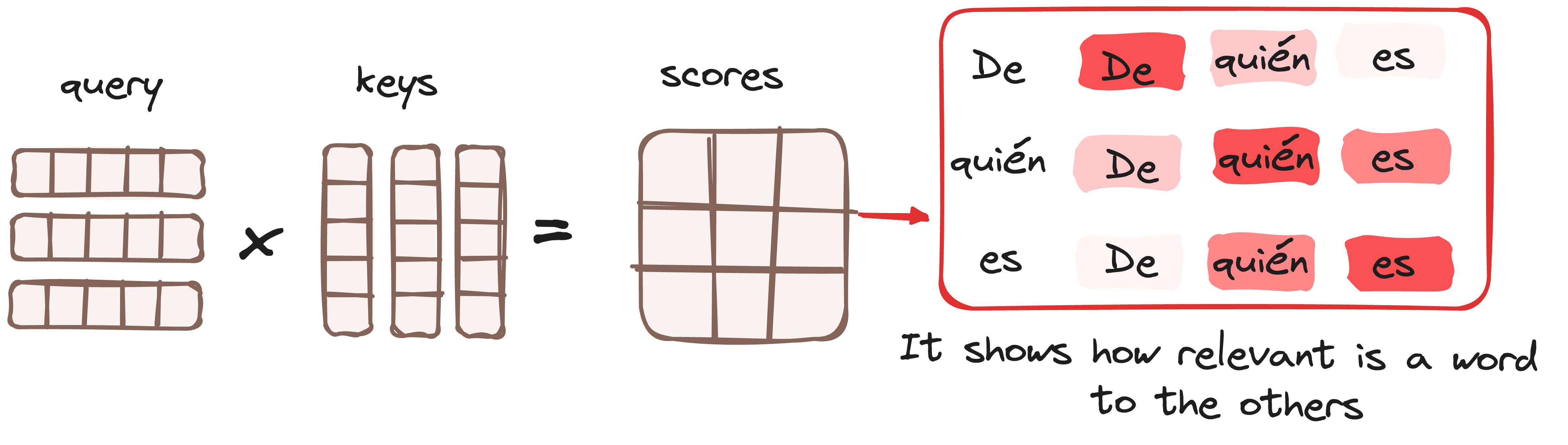
3.1.1 Matrix Multiplication (MatMul) - Dot Product of Query and Key
Once the query, key, and value vectors are passed through a linear layer, a dot product matrix multiplication is performed between the queries and keys, resulting in the creation of a score matrix.
The score matrix establishes the degree of emphasis each word should place on other words. Therefore, each word is assigned a score in relation to other words within the same time step. A higher score indicates greater focus.
This process effectively maps the queries to their corresponding keys.
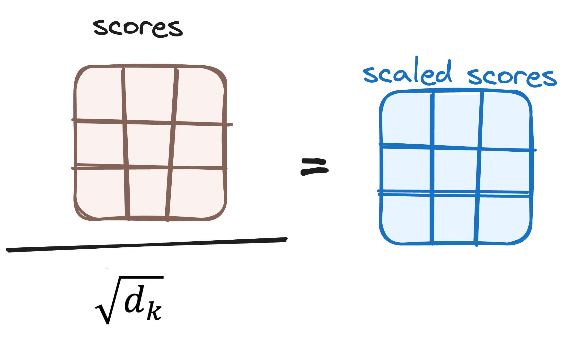
3.1.2 Reducing the Magnitude of attention scores
The scores are then scaled down by dividing them by the square root of the dimension of the query and key vectors. This step is implemented to ensure more stable gradients, as the multiplication of values can lead to excessively large effects.
3.1.3 Applying Softmax to the Adjusted Scores
Subsequently, a softmax function is applied to the adjusted scores to obtain the attention weights. This results in probability values ranging from 0 to 1.
The softmax function emphasizes higher scores while diminishing lower scores, thereby enhancing the model’s ability to effectively determine which words should receive more attention.

3.1.4 Combining Softmax Results with the Value Vector
The following step of the attention mechanism is that weights derived from the softmax function are multiplied by the value vector, resulting in an output vector.
In this process, only the words that present high softmax scores are preserved. Finally, this output vector is fed into a linear layer for further processing.

And we finally get the output of the Attention mechanism!
So, you might be wondering why it’s called Multi-Head Attention?
Remember that before the process starts, we break our queries, keys and values h times.
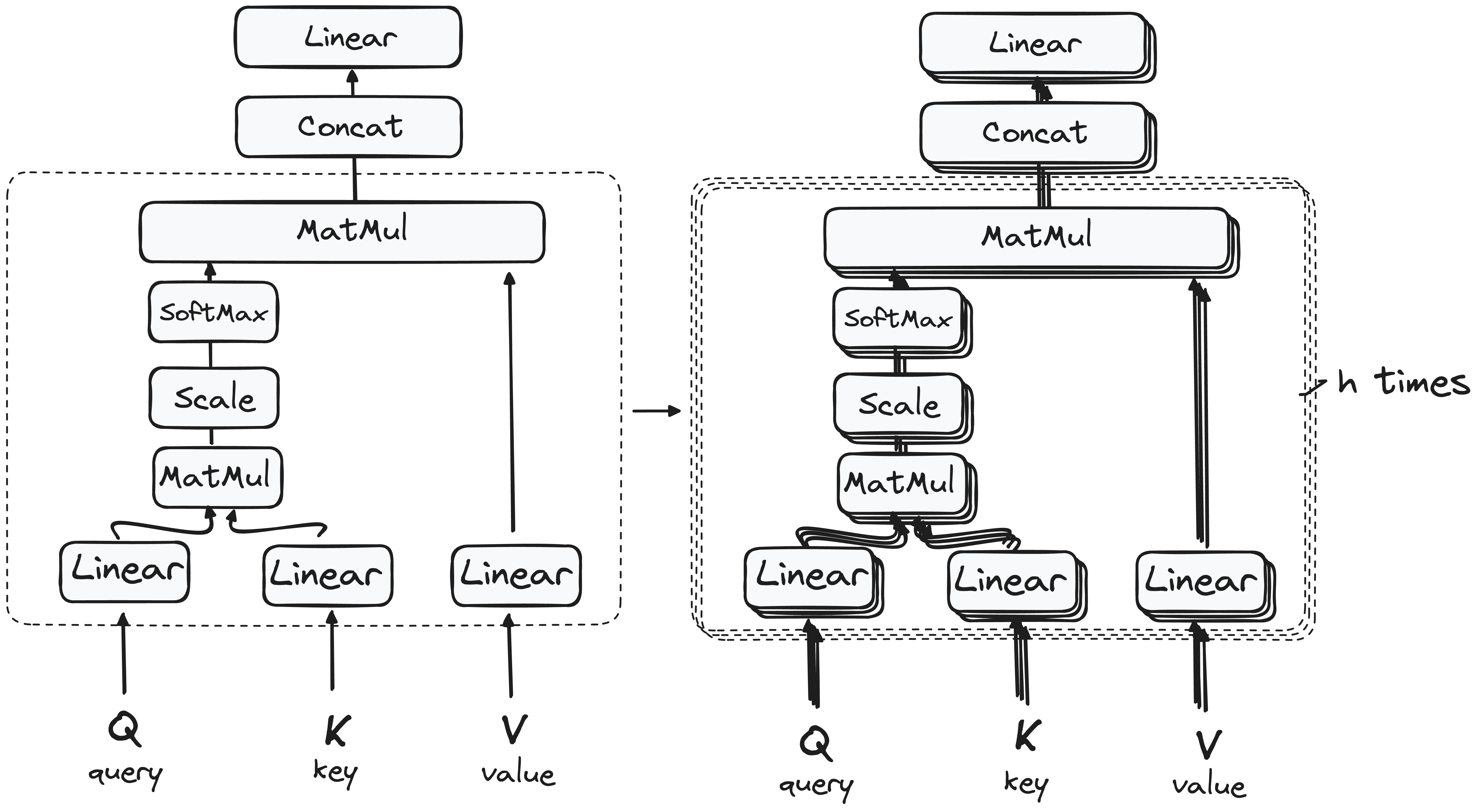
This process, known as self-attention, happens separately in each of these smaller stages or ‘heads’. Each head works its magic independently, conjuring up an output vector.
This ensemble passes through a final linear layer, much like a filter that fine-tunes their collective performance. The beauty here lies in the diversity of learning across each head, enriching the encoder model with a robust and multifaceted understanding.
STEP 3.2 Normalization and Residual Connections
Each sublayer in the encoder (self-attention and feed-forward) is followed by:
Residual Connections: The input of each sublayer is added to its output, mitigating gradient vanishing issues and facilitating deeper networks.
Layer Normalization: Helps stabilize training by standardizing activations, ensuring efficient learning.
This same process is applied after both self-attention and feed-forward layers, improving model performance.

STEP 3.3 Feed-Forward Neural Network
After attention processing, the sequence representation flows through a fully connected feed-forward network, refining the learned features.
This two-layer neural network consists of:
First Linear Layer: Expands the feature dimension.
ReLU Activation: Introduces non-linearity.
Second Linear Layer: Projects back to the original embedding size.
The output of the feed-forward network is then normalized and added to the residual connection, completing the transformation cycle.

STEP 4 - Output of the Encoder
After passing through multiple encoder layers, the final output is a set of contextualized vectors, each representing a token enriched with global sequence understanding.
This output serves as the input for the decoder, guiding it to generate relevant outputs by attending to specific encoder states.
Think of it as building a strong foundation, where each encoder layer contributes a new level of contextual refinement. The more layers, the richer and more abstract the representation becomes.
Wrapping Up the Encoder, Teasing the Decoder
Now that we’ve broken down the encoder, we’ve seen how it processes input sequences in parallel, capturing rich contextual representations that make Transformers so powerful.
But what happens next?
That’s where the decoder comes in.
Unlike the encoder, the decoder operates autoregressively, meaning it generates one token at a time while attending to both the encoded representations and its own past predictions. It also introduces a key difference—masked self-attention, which prevents the model from “peeking” at future tokens when generating text.
Next week, we’ll explore how the decoder builds on what the encoder has learned to generate coherent and meaningful sequences.
Stay tuned for our deep dive into the decoder!
—Josep
Are you still here? 🧐
👉🏻 I want this newsletter to be useful, so please let me know your feedback!
Before you go, tap the 💚 button at the bottom of this email to show your support, it really helps and means a lot!
Loading...
Any doubt? Let’s start a conversation! 👇🏻
Want to get more of my content? 🙋🏻♂️
Reach me on:
LinkedIn and X (Twitter) to get daily posts about Data Science.
My Medium Blog to learn more about Data Science, Machine Learning, and AI.
Just email me at rfeers@gmail.com for any inquiries or to ask for help! 🤓